Editor (Beta)

The Editor turns imported geometry into an asset that moves. A STEP or JT file arrives as a silent tree of CAD parts; the editor gives that tree axes, drives, materials and signals, and saves the result as a GLB that any realvirtual WEB document — and the Layout Planner — can reuse.

Unlike the other workspaces, the editor works on one asset document at a time rather than on a whole plant or layout. Every change is recorded as an undoable step, so authoring is a matter of trying something and looking at it, not of getting it right the first time.

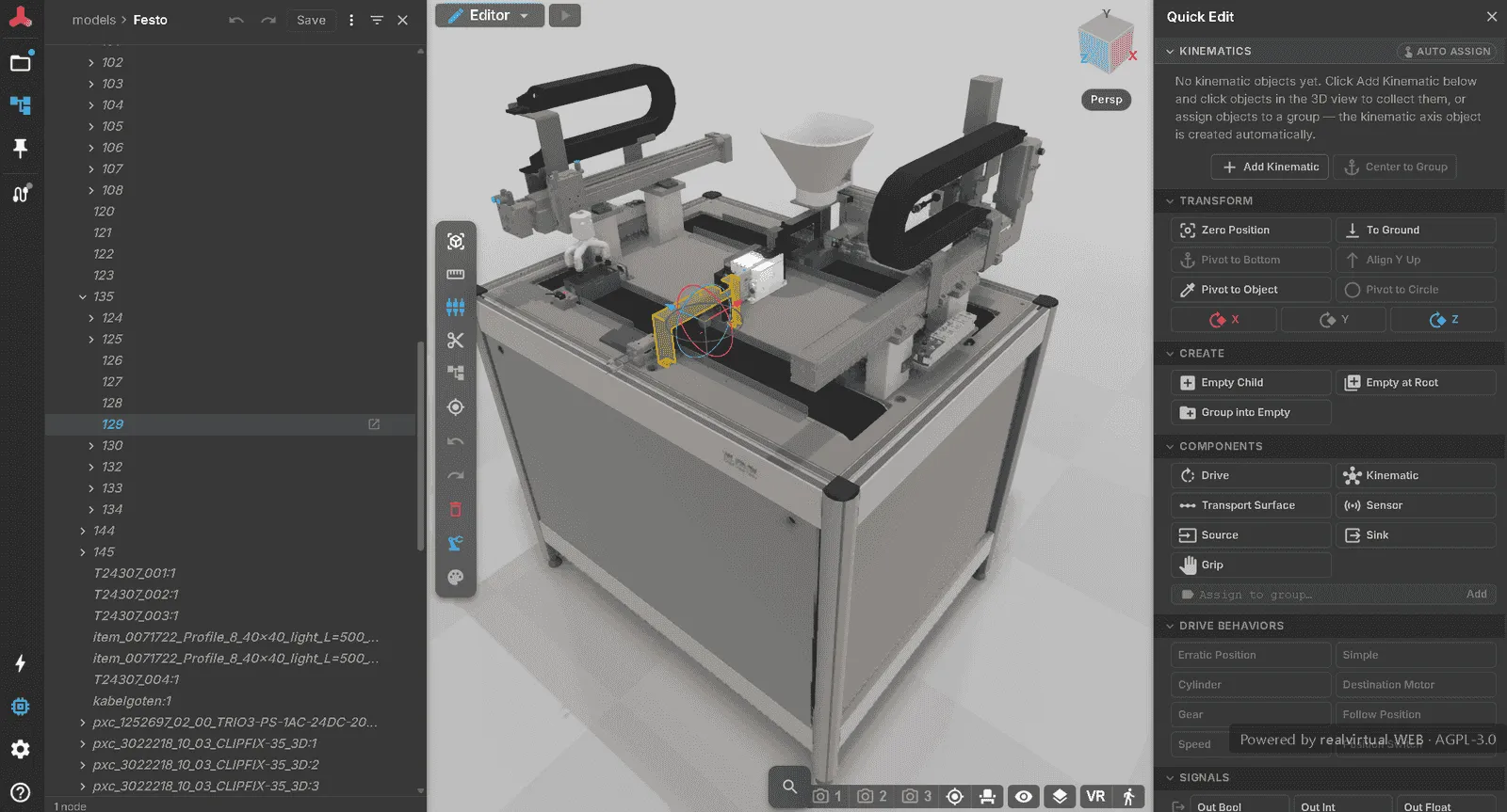
A Festo station open in the editor: the imported CAD tree with its original part names on the left, the tool strip and the transform gizmo in the 3D view, and Quick Edit with kinematics, transform, create, components, drive behaviours and signals on the right

Importing

Geometry arrives through one dialog with a tab per source — GLB, STEP, JT, USD, FBX, the Asset Manager and Onshape. Local files are read in the browser, and assemblies too large for a browser tab are converted by realvirtual CONNECT on the same machine. See importing CAD for the settings each source takes, the free-tier size limits, and how a CADLink node picks up a newer CAD revision.

The fastest way in is a link. ?doc=new&mode=editor creates a new asset in the open project (or in My Workspace when that project is read-only, such as the demo), opens it in the Editor and shows the import dialog straight away:

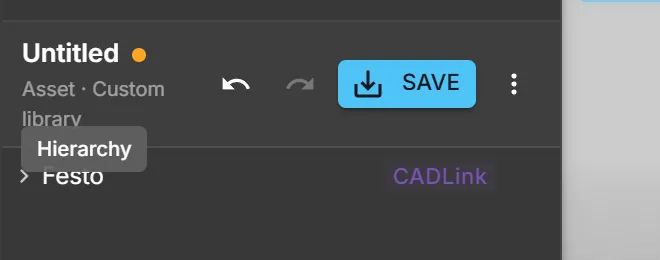
https://<your-deploy>/?doc=new&mode=editor

The document header shows what you are editing, whether it has unsaved changes, and the undo, redo and Save controls:

The asset header: name, unsaved marker, undo and redo, save

The Quick Edit panel

Quick Edit: kinematics, transform, create, components, drive behaviours, signals and logic steps

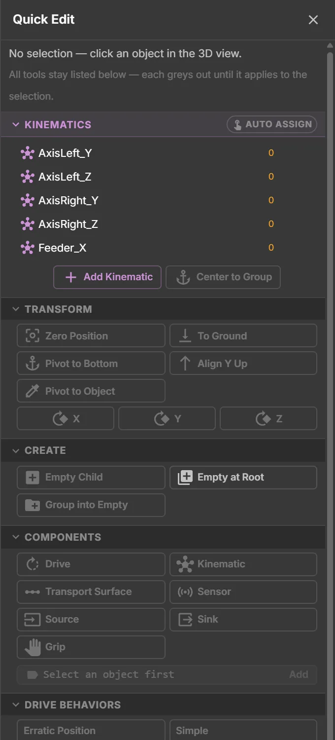
Everything you do to a selection happens here, and the panel is deliberately honest about it: every tool stays listed and greys out until it applies to what you have selected, so the set of available operations is always visible rather than appearing and disappearing.

Group	What it does
Kinematics	The axes of this asset, each with the number of parts assigned. Add Kinematic creates one from the current selection; Auto Assign proposes an assignment for the whole tree
Mechanism (Rigid-Body)	Closed-loop mechanisms — a four-bar coupler, a scissor lift, a Delta platform — built from Revolute, Prismatic, Spherical and Universal joints that solve together. Separate from Kinematics on purpose: see rigid-body mechanisms
Transform	Zero position, to ground, pivot to bottom, pivot to object, pivot to circle, align Y up, and rotation around X, Y or Z
Create	Empty child, empty at root, group into empty — the structure a raw CAD tree usually lacks
Components	Drive, Kinematic, Transport Surface, Sensor, Source, Sink, Grip
Drive Behaviors	Simple, Cylinder, Destination Motor, Gear, Follow Position, Speed, Position Switch, Erratic Position
Signals	Bool, Int and Float in both directions, plus conversions between them
Logic Steps	Sequences that drive the asset without a controller

In the example above, the imported Festo station already carries five axes — AxisLeft_Y, AxisLeft_Z, AxisRight_Y, AxisRight_Z and Feeder_X.

Pivot to Circle

A rotary axis turns around the centre of a bore, a bearing seat or a shaft — a point that is almost never the origin the CAD system left behind. Pivot to Circle puts the pivot on that centre by letting you point at the round feature instead of typing coordinates.

Select the part whose pivot you want to move and click Pivot to Circle.
Click the mesh that carries the round feature. The rest of the model dims and the camera frames what you picked, so the only thing competing for your attention is the geometry you are aiming at.
Move the cursor over the feature. The corner nearest the cursor lights up, and where that corner lies on a circle the circle is drawn together with the axis the commit would take.

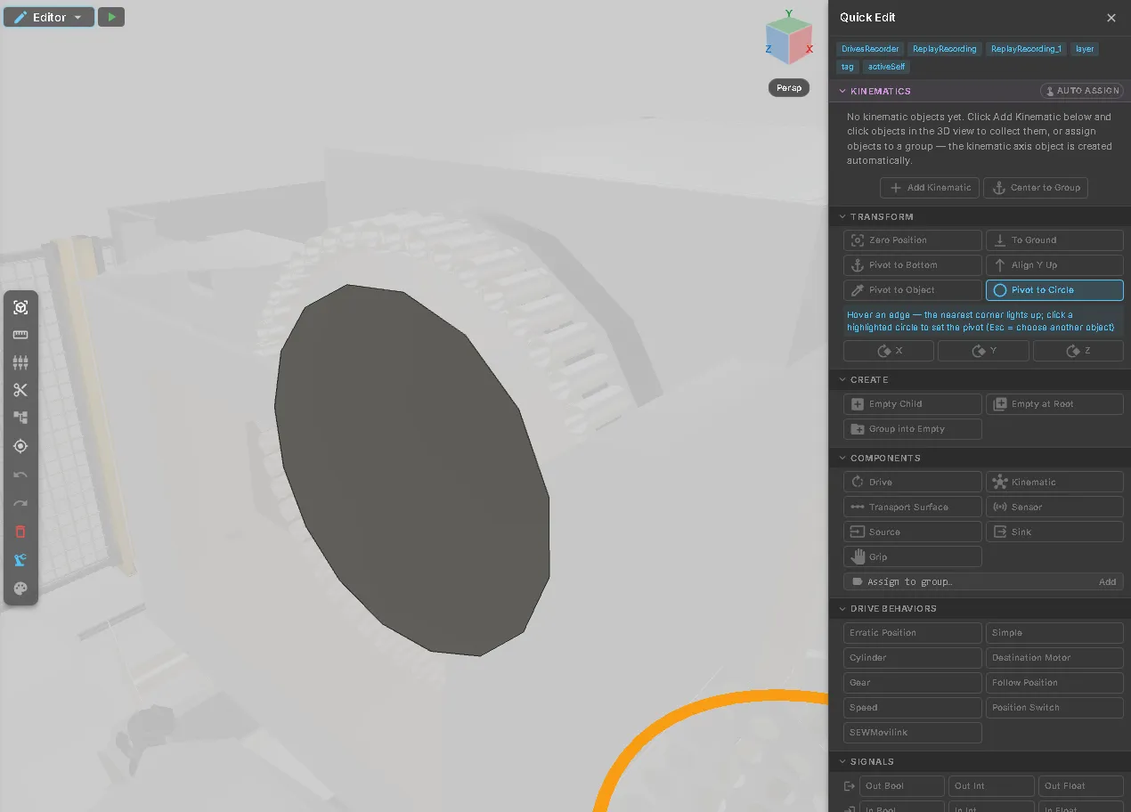Pivot to Circle at stage two: the picked mesh is framed and the rest of the cell is dimmed away, while Quick Edit keeps the Pivot to Circle button lit and prompts to hover an edge — the nearest corner lights up; click a highlighted circle to set the pivot 4. Click the circle to move the pivot there.

Escape steps back one stage rather than leaving the tool, because “wrong part” is the correction you will need most; Escape again, or a right-click, cancels. Every way out restores the normal view — the dim and the framing are part of the tool, not a state you can get stranded in.

Notes on a node

Any node can carry a written note — what the assembly does, how it is commissioned, what a maintainer needs to know. Notes are stored inside the document and travel with it, so they arrive with the machine rather than in a separate file. The property inspector renders a note as formatted text with a short header (when, by whom, how confident), in a box that grows with the window; long notes scroll inside it instead of stretching the panel.

Testing the asset

The ▶ button sits top-left next to the workspace dropdown, in the same place every other mode puts the control that starts time. It runs the asset you are authoring — drives, signals and logic steps — without leaving the editor and without saving first.

What the button starts is the real thing: pressing it exports the current authoring state through the same code path the Save button uses and loads the result back. Anything that behaves differently in a test run than after a save would be a save bug, not a test artefact.

While a run is live the group grows into the run controls the other workspaces use — Stop, Pause, Reset, a speed selector and the simulation clock. The two are not the same verb:

Stop ends the session: the test scene is dropped, the authoring state is restored exactly as it was, and the editing tools come back.
Pause only holds time inside the running session. The tools stay locked.

This is how you check an axis before committing to it. A wrong axis direction shows up as parts sliding instead of turning; a wrong pivot as an orbit instead of a spin.

Two consequences are worth knowing: Save is refused while a test run holds the document — stop the run first — and leaving the editor waits for the restore rather than cutting it short, so the authoring state is never half-swapped.

Saving

The document header carries the name, the unsaved marker and Save. A document is written back to where it came from, in the open project; Untitled is a name like any other, and only a document with no name at all is refused. A save that fails leaves no half-created document behind, and the card preview of a saved asset refreshes so the dashboard shows what you actually saved.

Save is refused while a test run holds the document — stop the run first. The full rules, including what happens when somebody else wrote the same file first, are under mesh and structure.

What you can do

Import — STEP, JT, USD, FBX and GLB, or geometry from Onshape, plus re-import of a newer CAD revision.
Structure — browse and rename the node tree, split and merge meshes, group parts, and work on nested assets.
Kinematics — group parts into an axis, add its drive, and place the rotation point. Rotary axes are defined in degrees, linear axes in millimetres.
Verification — run the asset in place and watch it move before saving (see Testing the asset).
Materials — assign from an industrial preset library (steel, RAL paints, rubber, glass) or set physical properties directly.
Signals and logic — add PLC input and output signals to nodes and connect simple sequences, so the asset reacts to live data or to a standalone simulation.
Forces — the toolbar’s Forces button opens the force and torque analysis for a rigid-body mechanism: actuator loads, bearing loads and the peak and RMS figures a drive has to be sized against. It is described in full under rigid-body mechanisms.

Quick Start

Switch the workspace to Editor — or open ?doc=new&mode=editor, which lands on the import dialog with a new asset already created.
Import a CAD file, or open an existing asset from the library.
Work out what the machine does — focus the camera on a part, select its identical copies, name what you see.
Group the parts of one movement into a kinematic axis and give it a drive.
Verify the axis by driving it through its range.
Assign materials.
Save. The asset lands in the library and can be placed, driven and connected like any other.

Where the result goes

A saved asset is an ordinary GLB with realvirtual metadata — the same format the Unity exporter produces and the same one the viewer reads. That means an asset authored in the browser is not a second-class citizen: it can be placed in a layout, connected to live signals through CONNECT, published as a document, or handed on as a file.

It lands in the project you are working in, and the project is itself the library the Layout Planner offers first. Nothing has to be published, registered or copied into a separate catalogue for a saved asset to be placeable — see documents for how libraries are attached.