Rigid-Body Mechanisms

Overview

A Delta picker open in the editor: the tree on the left shows the three driven arm axes above a DeltaMechanism node whose whole subtree is Kinematic Joints — revolute, universal and spherical — and the Kinematics list on the right holds the arms, the platform, the rods and the shaft as separate bodies

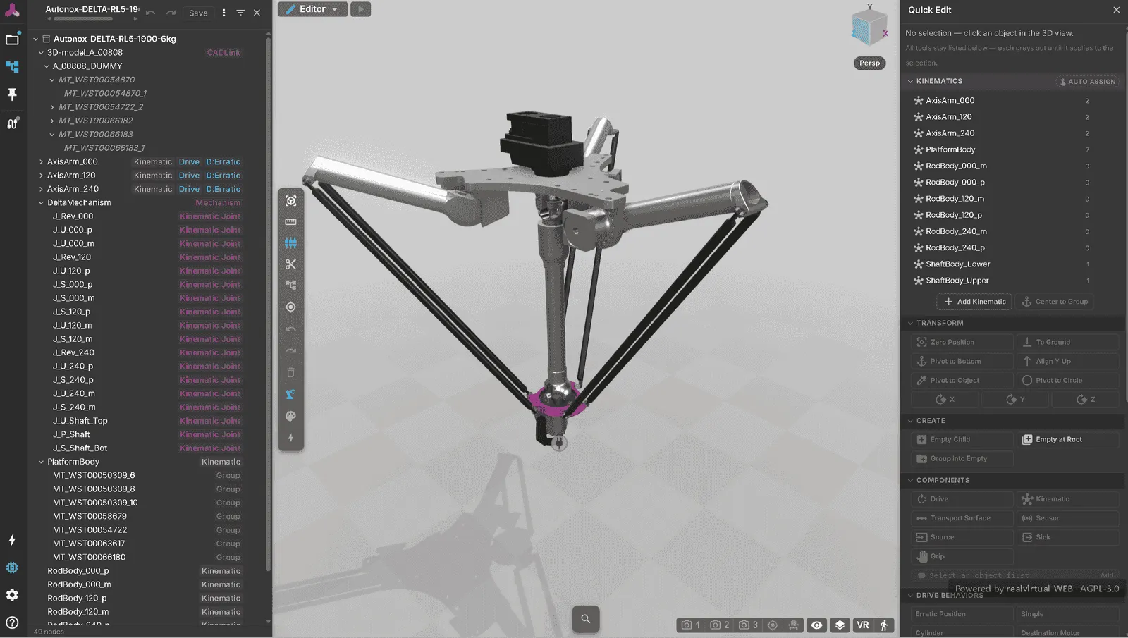
A rigid-body mechanism is a set of links connected by joints that solve together as one system, not as a chain of parent-child rotations. That is what makes closed loops possible — a four-bar coupler, a scissor lift, a Delta platform — where a link has to satisfy two joints at once and therefore cannot be the hierarchy child of both.

Two components make up a mechanism:

A Mechanism collects every joint in its subtree and runs the solver once per tick — a bounded, damped Newton-Raphson iteration that satisfies every joint simultaneously.
A Joint is one constraint between two links: Revolute, Prismatic, Spherical or Universal, with an anchor point and axis. Give a joint a Drive and it becomes a boundary condition the mechanism solves around; leave it undriven and the solver works out its value from the others.

An optional third component, a Target, runs the solve backwards: it drags a mechanism’s driven joints so that one of its own links follows a point in space — the way you’d want to move a Delta picker by dragging its platform rather than its three motors.

You get a mechanism one of two ways:

Build it in Unity. KinematicMechanism, KinematicJoint and KinematicTarget (Professional) author the same way any other kinematics does. Export to GLB and the mechanism runs identically in the viewer — Standalone simulation and Live mode both use the same solver as its Unity origin.
Build it in the browser. Quick Edit has a dedicated Mechanism (Rigid-Body) section for authoring one directly on raw, unkinematized CAD — no Unity round-trip required.

Not the same as Kinematics

The older Kinematics section in Quick Edit groups parts onto a single moving axis inside the existing hierarchy — the right tool for a hinge, a slide or a turntable. A mechanism instead solves a graph of joints, which is the only way to express a loop that closes back on itself. The two panels are intentionally kept apart and share no components: if what you’re building has one clear moving axis, use Kinematics; if it has a closed loop or several joints that move together, use Mechanism.

Key properties

Mechanism

Property	Description
Solver Iterations	Fixed number of Newton-Raphson iterations per tick (default 4). Kept constant for a deterministic solve.
Damping	Damped-least-squares factor that keeps the solve stable near a singular configuration (default 0.01).
Tolerance	Constraint residual, in millimeters, below which the solve counts as converged (default 0.001 mm).
Converged	Read-only. True when the last solve met the tolerance.
Residual Error	Read-only. The largest constraint error left after the last solve, in millimeters.

Joint

Property	Description
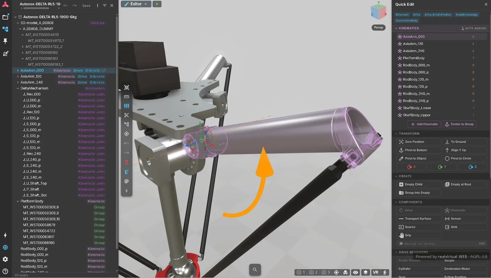
Joint Type	Revolute, Prismatic, Spherical or Universal. Only Revolute and Prismatic have a single scalar value, so only they can carry limits or a Drive.
Body A / Body B	The two links the joint connects. Leave Body A empty to anchor the joint against world space — that’s how you fix a mechanism to the machine frame instead of to another moving link. Body B is always required.
Anchor A / Anchor B	The joint’s pivot point, in each body’s own local space, in millimeters. The two should coincide in world space.
Axis A	The joint axis, in Body A’s local space. Unused by Spherical.
Secondary Axis B	A second axis in Body B’s local space, used only by Universal joints.
Use Limits / Lower / Upper Limit	Clamps the joint value in degrees (Revolute) or millimeters (Prismatic).
Driven By	The Drive that moves this joint. Leave it empty for a passive joint the mechanism solves for.
Current Value	Read-only. The joint’s live value, written by the solver every tick.

Target

Property	Description
Mechanism	The mechanism whose driven joints this target solves for.
Target Link	The mechanism’s own link that should follow this node — a Delta platform, for example.
Tracking Active	While on, an inverse solve runs every tick and takes over the mechanism’s Drives.
Reachable	Read-only. False when the target is outside the workspace or a limit was hit — the mechanism still moves to the closest pose it can reach.

Quick Start

From Unity

Build the mechanism with KinematicMechanism and KinematicJoint components, the same way as any Professional kinematics.
Export the scene to GLB.
Open the model in realvirtual WEB — the mechanism forward-solves exactly as it did in Unity, driven by the same Drives, in both Standalone and Live mode.

From the browser (Quick Edit)

Import the raw CAD and select the links you want to connect.
Open Mechanism (Rigid-Body) in Quick Edit and click + Mechanism.
Add a joint, pick its type, then click Body A and Body B directly in the 3D view — hover highlights the snap candidates (face centers, edges, circle centers) before you commit, and leaving Body A unset anchors the joint to the world.
Assign a Drive to the joint you want to move.
Validate and clear anything the findings list flags.
Jog the driven joint with its slider and watch the mechanism move under the real solver.
Save. The mechanism is part of the asset now, ready to place in a layout like any other component.

Assigning a Drive takes effect immediately: the running mechanism picks the Drive up on the next tick, so you can jog the joint straight away without reloading the model.

Snapping also reads curved surfaces. Hovering a bore or a cylindrical wall fits its axis and radius, so a revolute joint lands on the hole’s centerline instead of on the nearest flat feature — and when a bore and the boss around it are both under the cursor, the bore wins.

Validation & Jog

Every joint with a problem gets a warning next to it, naming the finding it triggered — a missing Body B, anchors that don’t coincide, a Drive whose axis doesn’t match the joint, and a few others. Where a fix is unambiguous, a Snap button applies it directly; everything else is diagnosis, not automation you have to trust blindly.

The Jog slider runs the actual solver, not a preview animation — the convergence flag and residual you see are what the mechanism will do at runtime. A configuration that doesn’t converge colors the joint and names the finding code responsible, so a limit conflict or an unreachable anchor shows up while you’re still building it, not after you’ve saved.

Force Analysis and Drive Sizing

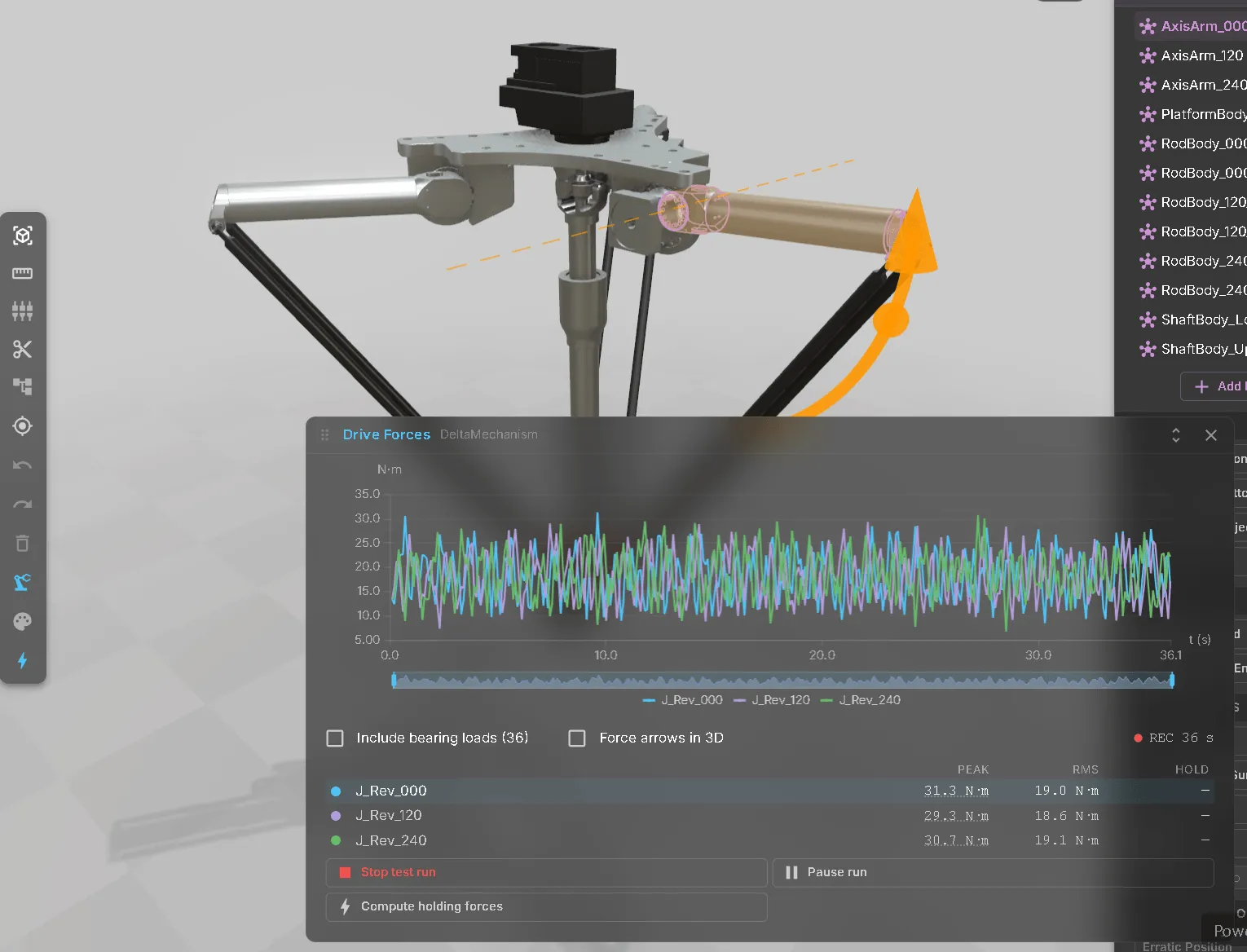
Once a mechanism moves, the next question is what it takes to move it. The same solver answers it: for every driven joint an actuator force or torque, and for every joint a bearing load. The motion is not affected — nothing on this path can change a pose.

Give each link a mass

Force analysis needs to know what it is moving, so every link of the mechanism needs a Body. Open the mechanism in Quick Edit and each link gets a row with an Add Body button:

Property	Description
Density Preset	Steel, aluminum, stainless, PA, POM or a custom value. The mass is computed from the link’s geometry and this density.
Mass	Read-only unless pinned. Shows the computed mass and how it was obtained — a value marked (estimated) came from a bounding box because the geometry was not closed.
Pin mass	Replaces the computed mass with the value you enter. Use it for a payload, for a part whose CAD is a placeholder, or for a link that carries no geometry at all.
COM	The center of mass in the link’s own coordinates. Pin it when the model omits something heavy — a motor, a cable carrier.

Two rules are worth knowing before you rely on a number:

The mass is never guessed silently. If a link’s geometry is open, self-intersecting or missing, the row says so and the value is labeled as an estimate.
One link without a usable mass switches the analysis off for the whole mechanism, and the findings list says which one. A partial answer would be worse than none: a drive sized against a machine that is missing its heaviest link is a drive that will not fit.

Record a cycle

Open Forces under the mechanism and press Test in the editor toolbar. The recording starts with the test run and ends when you stop it — the last cycle stays on screen so you can read it afterwards.

The chart plots every driven joint at once, one colour per joint with a legend under it — actuator torque for a rotary joint, force for a linear one. Include bearing loads adds the bearing series on top, with the number of them in brackets.
Peak is the largest magnitude over the cycle — the figure a drive has to survive once.
RMS is the effective value over the cycle, weighted by real elapsed time — the figure a drive has to survive continuously.
Hold is the holding torque in the current pose. It comes only from Compute holding forces, never from the recording — which is why the Hold column stays empty while a run is going: a moment where the velocity happens to pass through zero is not a machine standing still.

Both reference lines are drawn on the chart, so you can see at a glance whether a cycle is a short spike on a light duty or a sustained load.

Statics without running

Compute holding forces answers “what does it take to hold this?” in the pose the mechanism is in right now, with gravity and nothing moving. It needs no recording and no test run, which makes it the fastest way to check a lifting axis or a counterweight while you are still building the machine.

Force arrows in 3D

Tick Force arrows in 3D and every joint gets an arrow along its reaction force. Length is capped and the magnitude is in the color — scaling arrows linearly would push the loaded joint off screen and shrink every other one to nothing. Hovering an arrow reads out its value; clicking one selects that joint’s series in the chart. The arrows disappear when you leave the editor.

What it does not cover

No contact or process forces. Cutting forces, gripper contact and friction are not modeled. Represent a payload as an added mass on the link that carries it.
Where a mechanism is over-actuated — more drives than degrees of freedom in a loop — the split between the drives is not physically unique. The panel says so rather than quietly picking one.
Gravity is standard, along −Y. A tilted installation is not yet configurable.

Smooth (jerk-limited) motion

A drive that ramps with a constant acceleration changes that acceleration instantly at the start and end of the ramp. On a real machine that step is what shakes the structure, marks the product and wears the gearbox. Smooth motion replaces the trapezoidal ramp with a jerk-limited S-curve, so acceleration itself rises and falls at a bounded rate.

It is set on the drive, not on the mechanism, and applies just as much to an ordinary axis as to a joint the solver drives:

Property	Description
Use Acceleration	The existing acceleration ramp. Smooth motion is a sub-setting of it and does nothing on its own.
Smooth Acceleration	Switches the jerk-limited S-curve on in place of the trapezoidal ramp.
Jerk	The rate of change of acceleration, in mm/s³ for linear drives and deg/s³ for rotary ones. Lower is gentler and slower; higher approaches the hard trapezoidal ramp.
Speed Override	A factor on this drive’s speed, multiplied with the global simulation speed. It scales the time through the profile rather than the limits, so setting it to 0 pauses and resuming never makes the position jump.

The same numerical core runs in Unity and in the browser, so a machine that was tuned in Unity moves identically here — the S-curve exists once, not twice.

Where it is not available, a drive asking for smooth motion keeps running the familiar trapezoidal ramp and the viewer warns once for the model rather than once per drive. The model stays fully usable; it simply does not get jerk limiting. Endless rotary axes that wrap at their limits stay continuous across the wrap either way.

Drive behaviours and travel limits

This section is about a drive behaviour, which any drive can carry — a joint of a mechanism, or an ordinary axis that has nothing to do with one.

Erratic Position moves a drive to random positions between a minimum and a maximum — the quickest way to make an axis look busy in a demonstration or a load test.

Its range is clamped into the drive’s own travel limits. An authored range that reaches beyond them used to leave the axis parked forever, waiting for a position the drive would never hand back; now the target is clamped at the moment it is picked, and the viewer warns so the range can be corrected at the source. The return-to-zero on a falling enable signal is clamped the same way, which matters for an axis whose limits do not include zero.

Common Use Cases

Scissor Lift Table – A prismatic drive raises a platform through a chain of pivoting links.
Four-Bar Gripper – A single drive closes both jaws through a coupler link, keeping them synchronized without a second motor.
Delta Picker – Three arms constrain a platform to a Cartesian workspace; a Target lets you place the platform directly instead of driving each arm.
Slider-Crank – A rotary drive converts to linear motion (or back), the classic Prismatic + Revolute loop.